Understanding Flow Matching-based Generative Models

Recently, a series of concurrent works, Flow matching (Lipman et al., 2023), Rectified Flow (Liu et al., 2023), and Stochastic Interpolants (Albergo et al., 2023), proposed a new class of generative model based on Continuous Normalizing Flow (CNF), which we will refer to as Flow Matching (FM) based models. In principle, FM is a more flexible alternative to the current state-of-the-art Diffusion Models (DMs), and can be viewed as a generalization of DMs in two important ways:

• Trasport between arbitrary distributions:
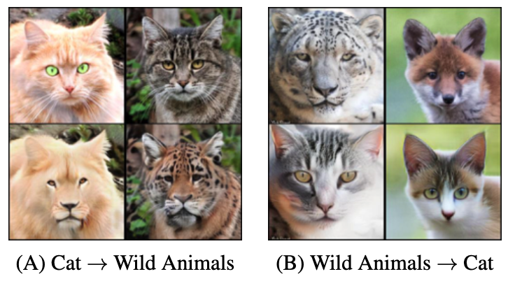
  DM requires the base probability distribution to be Gaussian. FM allows base distribtion to be any arbitrary distribution (e.g., image distribution). This can enable many applications such as image-to-image translations.
• Arbitrary probability paths:
  Path followed by DM is just one of the infinitely many possible probability paths that could be attained using FM models. This is important because it allows for flexible, application-specific designs of probability paths such as optimal transport path.

Normalizing Flow

FM can be seen as a subclass of the general flow based generative models. A flow model aims to transport a base distribution \(\rho_0\) to a target distribution \(\rho_1\), both defined over \(\mathbb{R}^d\), using a transport map \(\Psi: \mathbb{R}^d \to \mathbb{R}^d\), i.e., \[ \text{if } x_0 \sim \rho_0, \text{ then } \quad \Psi(x_0) \sim \rho_1. \] A popular framework, called the Normalizing Flow, learns such a transport map \(\Psi\) using maximum likelihood objective to learn a data distribution \(\rho_1\) by fixing the base distribution \(\rho_0\) to be a simple distribution, e.g., Gaussian, that is amenable to easy sampling and density evaluation. The objective of normalizing flow follows from the change of variable formula for probability density function as shown below: \[ \max_{\Psi} \quad \mathbb{E}_{x \sim \rho_1} \log p_{\Psi}(x):= \log \rho_0(\Psi^{-1}(x)) + \log |\det J_{\Psi^{-1}}(x)| \] As one can see, the above objective involves computing the determinant of the Jacobian of the inverse of the transport map \(\Psi\). For general functions \(\Psi\), this is a computationally prohibitive operation, especially for high-dimensional data. To avoid this expensive computation, \(\Psi\) is parameterized with a sequence of simple invertible transformations such that the Jacobian determinant is easy to compute. This restriction limited the expressiveness of normalizing flow models, consequently limiting their performance compared to other generative models such as GANs.

Continuous Normalizing Flow (CNF)

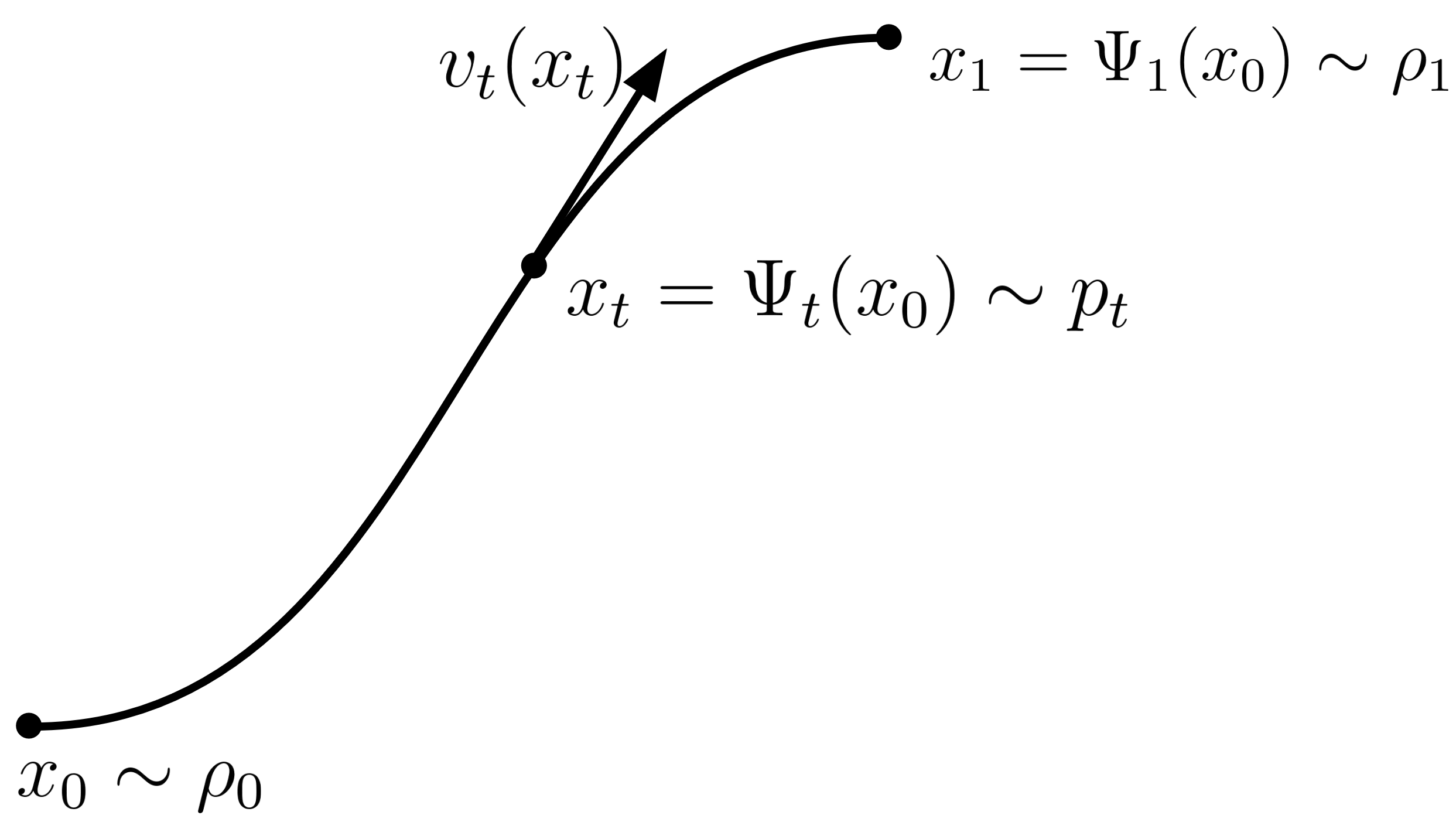
CNF uses a continuous time perspective of the aforementioned transport process. Consider a continuous time dependent map \(\Psi_t\) for \(t \in [0,1]\) such that \([\Psi_1]_{\# \rho_0} = \rho_1\) and \([\Psi_0]_{\# \rho_0} = \rho_0\), a time-dependent velocity field, \(v_t: \mathbb{R}^d \to \mathbb{R}^d\), and corresponding time-dependent probability path \(p_t: \mathbb{R}^d \to \mathbb{R}_{>0}\). The vector field \(v_t\) is related to the transport map \(\Psi_t\) via the following ordinary differential equation (ODE): \[ \frac{d}{dt} \Psi_t(x) = v_t(\Psi_t(x)). \] And the time-dependent probability path \(p_t\) is related to end distributions via: \[ p_t = [\Psi_t]_{\# \rho_0} \]

Mass Continuity Equation

A velocity field \(v_t\) results in the probability path \(p_t\) if and only if it satisfies the mass continuity equation: \[ \frac{\partial p_t}{\partial t} + \nabla \cdot (p_t v_t) = 0. \] This equation follows from Gauss's divergence theorem by enforcing probability mass conservation. Basically, one can use this equation to verify if a vector field \(v_t\) generates a given probability path \(p_t\), or to even find such a vector field (which is what we will do).

Flow Matching (FM)

Given a probability density path \(p_t\) with \(p_0 = \rho_0, ~p_1 = \rho_1 \), and corresponding vector field \(u_t\), the flow matching objective is to minimize the following loss function: \[ \mathcal{L}_{\rm FM}(v_t) = \mathbb{E}_{t \sim \mathcal{U}([0,1]), x \sim p_t} \|v_t(x) - u_t(x)\|^2. \] \(\mathcal{L}_{\rm FM}\) is simple but intractable in practice as it requires access to two quantities that we have no prior knowledge on: (i) samples from \(p_t, \forall t\) and (ii) the vector field \(u_t\). In the following sections, we will discuss how to solve the two problems, (i) and (ii), to make the flow matching objective practical.

Stochastic Interpolant

In (Albergo et al., 2023), the authors define a time differentiable interpolant function \[ I_t:\mathbb{R}^d \times \mathbb{R}^d \to \mathbb{R}^d, ~t \in [0,1]\] such that \[ I_{t=0}(x_0, x_1) = x_0, \quad I_{t=1}(x_0, x_1) = x_1.\] A typical example of \(I_t\) is the linear interpolant: \[ I_t(x_0, x_1) = (1-t)x_0 + tx_1.\] Next, a joint distribution (coupling) \(\rho(x_0, x_1)\) is chosen such that \[ \int \rho(x_0, x_1) dx_0 = \rho_1(x_1), ~ \text{and } ~ \int \rho(x_0, x_1) dx_1 = \rho_0(x_0).\] The independent coupling \( \rho(x_0, x_1) = \rho_0(x_0)\rho_1(x_1)\) is a special example that satisfies the above conditions. The final tractable flow matching objective takes the following form: \[ \mathcal{L} = \mathbb{E}_{t, (x_0,x_1) \sim \rho(x_0,x_1), x = I_t(x_0,x_1)} \left\|v_t(x) - \frac{\partial}{\partial t}I_t(x_0,x_1) \right\|^2 \] For the linear interpolant \(I_t(x_0,x_1) = (1-t)x_0 + tx_1\) and independent coupling the above objective becomes: \[ \mathcal{L} = \mathbb{E}_{t, x_0 \sim \rho_0, x_1 \sim \rho_1, x = (1-t)x_0 + tx_1} \left\|v_t(x) - (x_1 - x_0) \right\|^2 \] The above objective is very simple to implement: one just needs to randomly sample a \(x_0\) and \(x_1\) from the two datasets, a time stamp and regress the vector field at \(I_t(x_0,x_1)\) with a vector pointing from \(x_0\) to \(x_1\). At first glance, it almost seems too simple and naive: how can matching the vector field with random directions recover the desired vector field \(u_t\)? The short answer is that, in expectation, these random directions will recover the desired vector field \(u_t\). To understand why this is the case, the following section will guide you through the detailed proof.

Proof:

(i) Sampling from \(p_t\)

1. Sample \((x_0,x_1) \sim \rho(x_0,x_1)\)
2. Compute \(x_t = I_t(x_0,x_1)\). \(x_t\) is our required sample.

(ii) Estimating \(u_t\)

Note on Diffusion Model

Diffusion model (stochastic or deterministic/probability flow) can be viewed as a special case of flow matching. Consider a special instance of interpolant function \(I_t(x_0, x_1) = \alpha_t x_0 + \sigma_t x_1 \). Further, let \(\rho_0 = \mathcal{N}(0,1)\). Then Variance preserving (VP) SDE follows the probability path determined by \(\sigma_t = \sqrt{1-\alpha_t^2}\), where \( \alpha_t = \exp(-\frac{1}{2}\int_0^t \beta(s) ds) \), and \(\beta\) is the noise schedule function.

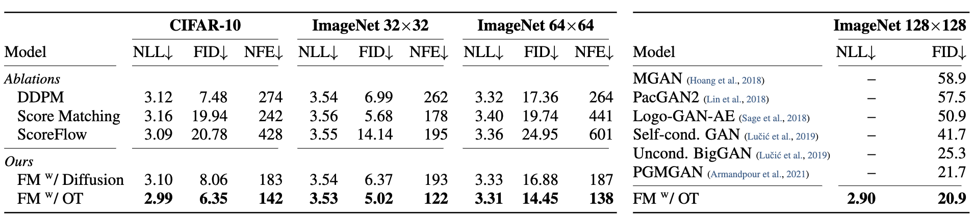
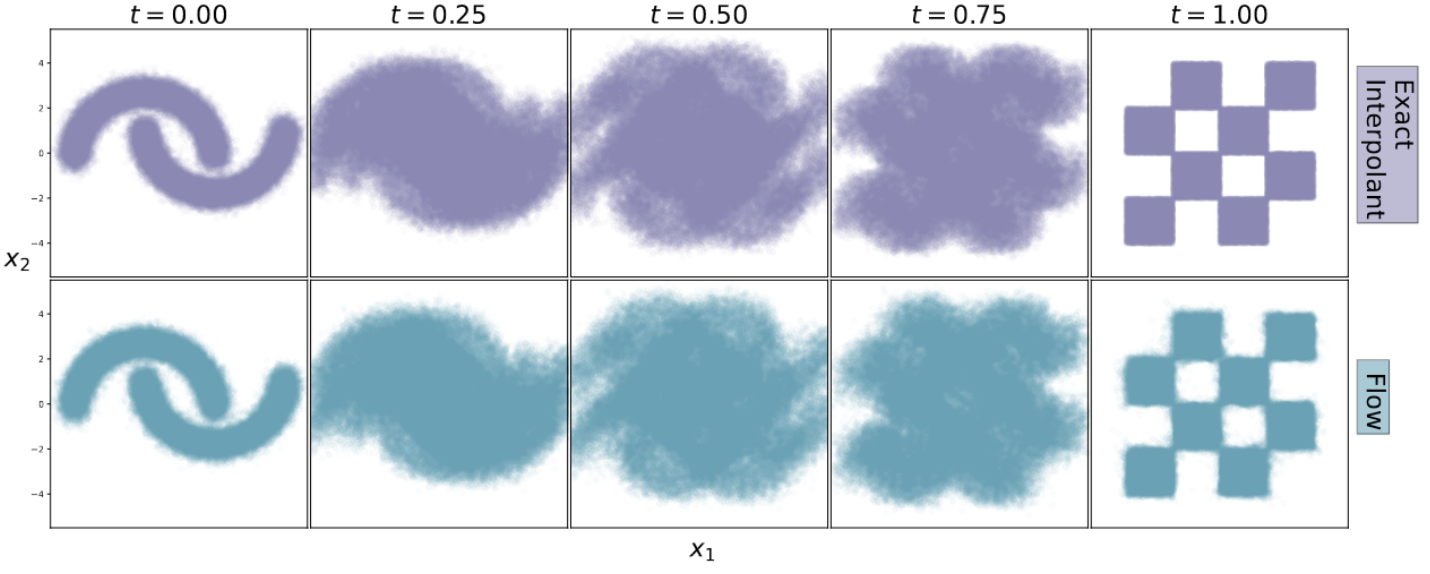
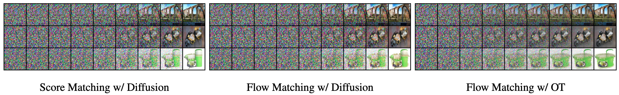
Results

References

[Lipman et al., 2023] Lipman, Y., Chen, R. T., Ben-Hamu, H., Nickel, M., & Le, M. (2023). Flow matching for generative modeling. arXiv preprint arXiv:2210.02747.
[Chen et al., 2018] Chen, R. T., Rubanova, Y., Bettencourt, J., & Duvenaud, D. K. (2018). Neural ordinary differential equations. Advances in neural information processing systems, 31.
[Albergo et al., 2023] Albergo, M. S., & Vanden-Eijnden, E. (2023). Building normalizing flows with stochastic interpolants. arXiv preprint arXiv:2209.15571.
[Liu et al., 2023] Liu, X., Gong, C., & Liu, Q. (2023). Flow straight and fast: Learning to generate and transfer data with rectified flow. arXiv preprint arXiv:2209.03003.