Unified Perspective on Diffusion and Flow Matching

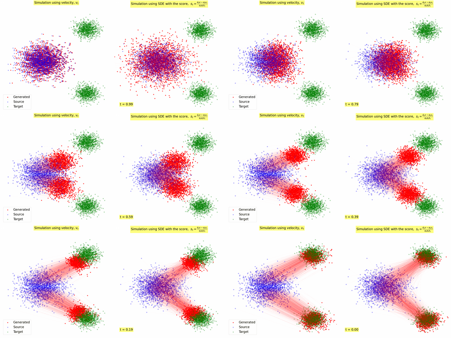
Diffusion and Flow matching are the state-of-the-art generative models for generating high-quality and diverse data in many domains (e.g., images, audio, video, graph, etc). They are appealing for two main reasons:

• They have simple least squares minimization training objectives, in contrast to the min-max optimization of GANs, therefore they are easier to train and scale to large datasets and models.
• They can generate high-quality and diverse data samples.

Despite their popularity and wide applicability, diffusion and flow matching models remain challenging for newcomers to fully grasp, particularly in terms of their intricate relationships. The literature presents diffusion models from various angles, such as denoising diffusion probabilistic models (DDPM) and denoising score matching. Flow matching, on the other hand, is often viewed as a distinct category of generative models, drawing inspiration from normalizing flows. This blog post aims to elucidate a unified perspective on diffusion and flow matching models, offering a clearer, more concise, and comprehensive understanding of both frameworks. Additionally, we'll explore how to flexibly transition between these approaches, providing a more holistic view of these powerful generative techniques.

1. The Density Transport Perspective

Both diffusion and flow matching fall under continuous normalizing flow based generative models [Lipman et al., 2023]. The main idea is to continuously morph one distribution \(p_0\) to another \(p_T\). Diffusion models can be regarded as a special case of flow matching where one of the distributions, i.e., \(p_T\), is a simple easy-to-sample distribution, such as a Gaussian, and the other distribution \(p_0\) is the data distribution. Whereas in flow matching, both \(p_0\) and \(p_T\) are allowed to be data distributions (Note: We follow notation convention in diffusion models where the ultimate goal is to transport samples from \(p_T\) to \(p_0\); generally, flow matching literature uses the reverse direction).

1.1. Probability Path and Stochastic Process

Both diffusion and flow matching can be characterized by a continuous time-dependent probability distribution \(p_t, t \in [0, T]\) that changes smoothly between \(p_0\) and \(p_T\). In general, \(p_t\) is defined as a sequenece of probability distributions associated with the random process \(\bar{x}_t\) defined as follows: \[ \bar{x}_t := I(x_0, x_R, t), \text{ such that } x_0 \sim p_0, x_R \sim p_R. \tag{1} \] where \(I(x_0, x_R, t)\) is an interpolating function that is differentiable with respect to \(t\) and \(p_R\) is a reference distribution which is closely related to \(p_T\). \(\bar{x}_t\) is constructed in such a way that \begin{align*} \bar{x}_{t=0} &= x_0 \sim p_0, \\ \bar{x}_{t=T} &\sim p_T. \end{align*} In practice, both flow matching and diffusion models generally select \(I(x_0, x_T, t)\) to follow the following form: \begin{align} \bar{x}_t = I(x_0, x_R, t) = \alpha(t) x_0 + \sigma(t) x_R, \tag{2} \end{align} where \(\alpha(t)\) is a smooth decreasing function of time \(t\) and \(\sigma(t)\) is a smooth increasing function of time \(t\).

Flow-matching uses the following setting:

• \(x_R = x_T \sim p_T\)
• \(\alpha(0) = 1\) and \(\alpha(T) = 0\)
• \(\sigma(0) = 0\) and \(\sigma(T) = 1\)
• \(T=1\)

Diffusion models generally uses the following setting:

• \(x_R \sim \mathcal{N}(0, I)\)
• \(p_T\) is a Gaussian distribution with variance \(\sigma(T)^2 I\), i.e., \(p_T = \mathcal{N}(0, \sigma(T)^2 I)\)
• \(T\) is large enough such that \(\bar{x}_{t=T} \) approaches \(p_T = \mathcal{N}(0, \sigma(T)^2 I)\).

2. Flow Matching

2.1. Flow and the velocity field

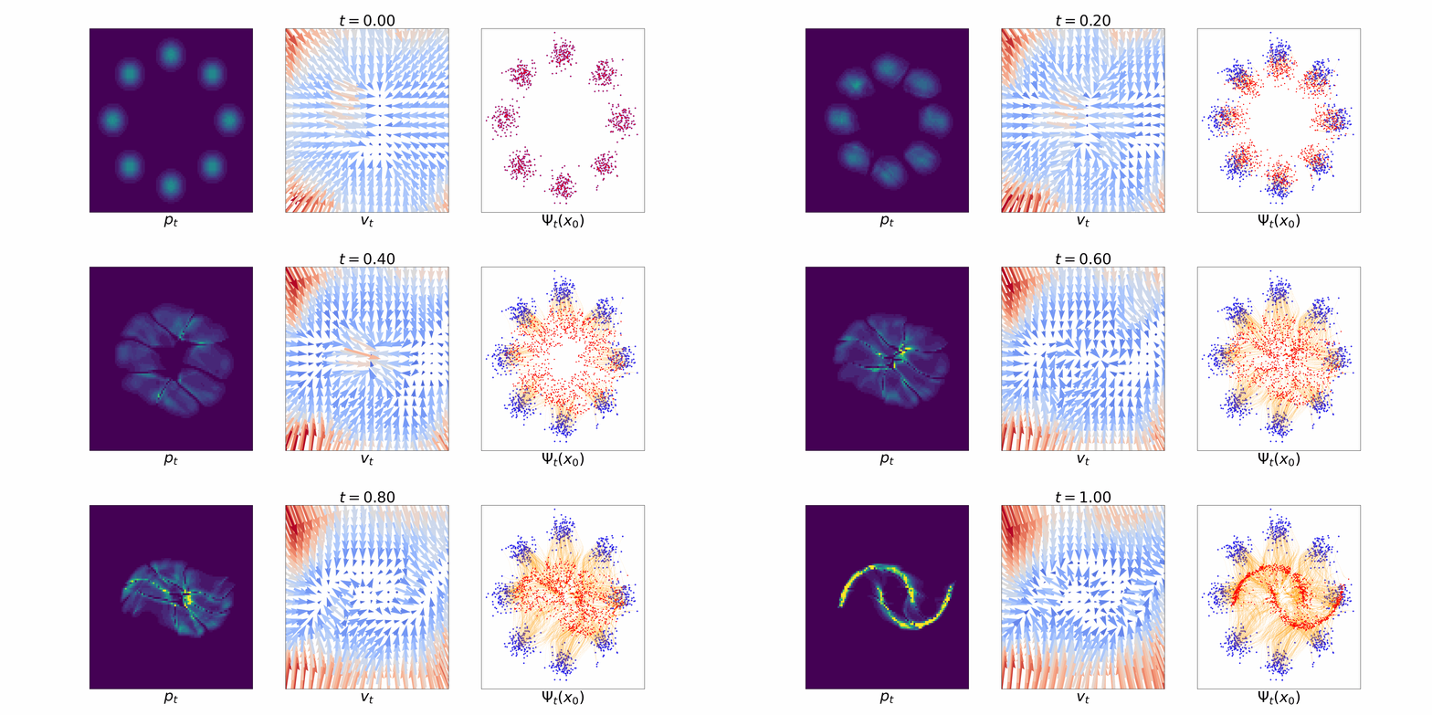
Figure 1: [Left] Evolution of \(p_t\); [Middle] time dependent velocity field \(u_t\); [Right] time dependent flow \(\Psi_t\).

Flow matching is inspired by normalizing flow based generative models [Papamakarios et al., 2021]. There the idea is to estimate an invertible map \(\Psi: \mathbb{R}^d \to \mathbb{R}^d\), called a flow, that maps samples from \(p_0\) to that from \(p_T\), i.e., \(x_0 \sim p_0 \implies \Psi(x_0) \sim p_T\), and vice versa, i.e., \(x_T \sim p_T \implies \Psi^{-1}(x_T) \sim p_0\). However, directly estimating such a map is challenging [Flow matching blog]. Continuous normalizing flow [Chen et al., 2018] was proposed to circumvent the need for estimating the flow \(\Psi\) by instead defining a differentiable time-dependent flow \(\Psi_t\) for \(t \in [0, T]\) such that the final flow at \(t = T\) is the desired map \(\Psi = \Psi_T\). This time dependent flow is related to the probability path \(p_t, t \in [0, T]\) as \[\Psi_t(x_0) \sim p_t, ~ t \in [0, T]. \] Such a time-dependent flow \(\Psi_t\) can be characterized by a time-dependent vector field \(u_t: \mathbb{R}^d \to \mathbb{R}^d\), also called the velocity field, defined as \[ u_t(\Psi_t(x_0)) = \dot{\Psi}_t(x_0), \] where \(\dot{\Psi}_t(x_0) = \frac{\partial}{\partial t} \Psi_t(x_0)\).

Denoting \(\Psi_t(x_0) = x_t\), we can rewrite the above as the following Ordinary Differential Equation (ODE): \[ dx = u_t(x) dt. \tag{3} \]

Given \(u_t\), one can simply transport samples between \(p_0\) and \(p_T\) by integrating the velocity \(u_t\) using an off-the-shelf ODE solver. For example, to transport a sample \(x_0 \sim p_0\) to \(x_T \sim p_T\), one can use simple Euler's method to obtain the following update rule: \[ x_{t + \Delta t} = x_t + u_t(x_t) \Delta t. \]

2.2. The flow matching objective

Flow matching (FM) aims at estimating the velocity field \(u_t\) that continuously morphs \(p_0\) to \(p_T\) tracing the probability path \(p_t, t \in [0, T]\). The ideal flow matching objective is to estimate the true velocity field \(u_t\) by solving the following least squares objective. \[ \min_{\theta} ~~\mathcal{L}_{\text{FM}}(\theta) = \mathbb{E}_{x_t \sim p_t} \left[ \left\| v_\theta(x_t, t) - u_t(x_t) \right\|^2 \right]. \tag{4} \] However, this ideal objective is intractable because the true velocity field \(u_t\) is unknown. Instead, FM considers the following conditional flow matching objective, which has the same minimizer as that of Eq. (4) [Lipman et al., 2023, Albergo et al., 2023, Liu et al., 2023] [my FM blog]: \[ \min_{\theta} ~~\mathcal{L}_{\text{CFM}}(\theta) = \mathbb{E}_{z \sim q(z), x_t \sim p_t(x_t|z)} \left[ \left\| v_\theta(x_t, t) - u_t(x_t|z) \right\|^2 \right], \tag{5} \] where \(z\) is any conditioning information, and \(u_t(x_t|z)\) is the conditional velocity field that traces the conditional probability path \(p_t(x_t|z)\) for a given \(z\).

A common choice of \(z\) is the endpoints \([x_0, x_1]\), with \(q(z) = \rho(x_0, x_T)\) being any joint distribution of \( x_0, x_T \) with the correct marginals \(p_0\) and \(p_T\). With this choice of \(z\), one can set \(p_t(x_t|x_0, x_T)= \delta_{I(x_0, x_T, t)} (x_t)\), where \(\delta_y(x)\) is the Dirac measure centered at \(y\), and \(I(x_0, x_T, t)\) is the interpolant function defined in Eq. (1). This will imply that \(u_t(x_t|z) = u_t(x_t|x_0, x_T) = \frac{\partial}{\partial t} I(x_0, x_T, t)\) is the associated unique conditional vector field. Hence, the practical objective used throughout the FM literature is given by: \[ \min_{\theta} ~~\mathcal{L}_{\text{CFM}}(\theta) = \mathbb{E}_{t, (x_0, x_T) \sim \rho(x_0, x_T)} \left[ \left\| v_\theta(I(x_0, x_T, t), t) - \frac{\partial}{\partial t} I(x_0, x_T, t) \right\|^2 \right]. \tag{6} \]

The optimal solution of Eq. (6), assuming expressive enough function class for \(v_\theta\), is given by: \[ v_{\theta^\star}(x, t) = \mathbb{E}_{(x_0, x_T) \sim \rho(x_0, x_T)} \left[ \dot{I}(x_0, x_T, t) ~\Big|~ x = I(x_0, x_T, t) \right]. \tag{7} \] Substituting the realization of \(I(x_0, x_T, t)\) from Eq.(2) into Eq. (7), and representing \(I(x_0, x_T, t)\) as \(\bar{x}_t\), we get: \[ v_{\theta^\star}(x, t) = \mathbb{E}_{(x_0, x_T) \sim \rho(x_0, x_T)} \left[ \dot{\alpha}(t) x_0 + \dot{\sigma}(t) x_T ~|~ x = \bar{x}_t \right]. \tag{8} \] Since \(\alpha(t)\) and \(\sigma(t)\) are constants with respect to \(x_0\) and \(x_T\), we can further simplify Eq. (8) as: \[ v_{\theta^\star}(x, t) = \dot{\alpha}(t) \mathbb{E}[x_0 ~|~ x = \bar{x}_t] + \dot{\sigma}(t) \mathbb{E}[x_T ~|~ x = \bar{x}_t]. \tag{9} \]

Eq. (9) suggests that the only data-dependent quantities that the optimal vector field depends upon are the conditional means \(\mu_0 = \mathbb{E}[x_0 ~|~ x = \bar{x}_t]\) and \(\mu_T = \mathbb{E}[x_T ~|~ x = \bar{x}_t]\). The conditional means will reappear in the next section on diffusion models, and will allow us to express the vector field in terms of the score (or denoiser) and vice versa.

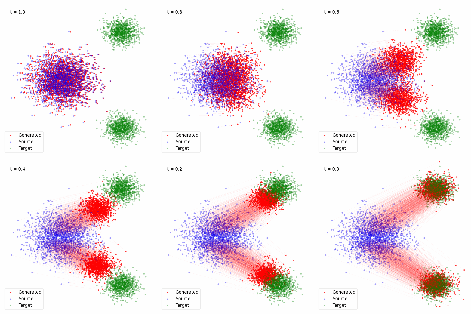
Figure 2: Trajectory of the samples following the vector field \(v_{\theta^\star}(x, t)\), the solution of Eq. (6) for \(\alpha(t) = 1- t, \sigma(t) = t\).

2.3. Flow Matching Implementation

Here's a simple Python implementation of the Flow Matching objective using PyTorch which was used to generate Figure 2:

import torch
import torch.nn as nn
import torch.optim as optim
from torch.utils.data import DataLoader, TensorDataset
from sklearn.datasets import make_blobs
import numpy as np
import matplotlib.pyplot as plt
from tqdm import tqdm

# Hyperparameters
batch_size = 512
epochs = 200
learning_rate = 1e-3

# Generate two Gaussians dataset in corners (4,4) and (4,-4)
X, _ = make_blobs(n_samples=10000, centers=[(4,4), (4,-4)], cluster_std=0.5, random_state=42)
X = torch.tensor(X, dtype=torch.float32)

# Simple MLP model for vector field
class VectorFieldMLP(nn.Module):
    def __init__(self):
        super().__init__()
        self.net = nn.Sequential(
            nn.Linear(2 + 1, 64),
            nn.ReLU(),
            nn.Linear(64, 64),
            nn.ReLU(),
            nn.Linear(64, 2)
        )

    def forward(self, x, t):
        x = torch.cat([x, t], dim=-1)
        return self.net(x)

def compute_alpha_t(t):
    return 1 - t, -1

def compute_sigma_t(t):
    return t, 1

# Training function
def train(model, dataloader, optimizer, device):
    model.train()
    total_loss = 0
    for x_0 in tqdm(dataloader):
        x_0 = x_0[0].to(device)
        optimizer.zero_grad()

        # Generate noise
        x_1 = torch.randn_like(x_0)
        
        # Sample t uniformly
        t = torch.rand(x_0.shape[0], device=device)
        t = t.unsqueeze(-1)
        alpha_t, d_alpha_t = compute_alpha_t(t)
        sigma_t, d_sigma_t = compute_sigma_t(t)
        # Interpolate between x_0 and x_1
        x_t = alpha_t * x_0 + sigma_t * x_1
        
        # Compute vector field
        v_theta = model(x_t, t)
        
        # Compute loss
        loss = torch.mean(torch.sum((v_theta - (d_alpha_t * x_0 + d_sigma_t * x_1))**2, dim=-1))

        loss.backward()
        optimizer.step()
        
        total_loss += loss.item()
    
    return total_loss / len(dataloader)


# Initialize model, optimizer, and dataloader
device = torch.device("cuda" if torch.cuda.is_available() else "cpu")
model = VectorFieldMLP().to(device)
optimizer = optim.Adam(model.parameters(), lr=learning_rate)
dataloader = DataLoader(TensorDataset(X), batch_size=batch_size, shuffle=True)

# Training loop
losses = []
for epoch in range(epochs):
    loss = train(model, dataloader, optimizer, device)
    losses.append(loss)
    if (epoch + 1) % 50 == 0:
        print(f"Epoch {epoch+1}/{epochs}, Loss: {loss:.4f}")


def static_sample(model, num_samples, device, source_samples, num_steps=100):
    # Convert source samples to tensor and move to device
    x = torch.tensor(source_samples, dtype=torch.float32).to(device)

    # Time steps
    dt = 1 / num_steps

    with torch.no_grad():
        # Euler integration
        for frame in range(num_steps):
            t = torch.ones(num_samples, device=device) * (1 - frame * dt)
            t = t.unsqueeze(-1)
            v = model(x, t)
            x = x - v * dt

    return x.cpu().numpy()
        

3. Diffusion Models

3.1. Instances of the diffusion process

In diffusion models, the continuous morphing of \(p_0\) to \(p_T\) is called the forward diffusion process, whereas the reverse direction from \(p_T\) to \(p_0\) is called the reverse diffusion process. The forward diffusion is a random process in which a Gaussian noise is gradually added to the data \(x_0 \sim p_0\) as follows: \[ \bar{x}_t = I(x_0, \epsilon, t) = \alpha(t) x_0 + \sigma(t) \epsilon, ~ \epsilon \sim \mathcal{N}(0, I), \tag{10}\] where \(\sigma(t)\) is a monotonically increasing function of \(t\) and \(\alpha(t)\) is a non-increasing function of \(t\). Note that we replaced \(x_T\) with \(\epsilon\). The choices of \(\alpha(t), \sigma(t), T\) are made in such a way that at \(t = T\), the variance of the second term \(\sigma(t)\epsilon\) in Eq. (10) dominates, and thus \(\bar{x}_T\) is distributed approximately as \(\mathcal{N}(0, \sigma(t)^2 I)\).

Different choices of the noise schedule \(\alpha_t, \sigma_t\) will give different instances of the diffusion process. Two notable instances are the variance preserving (VP) diffusion [Ho et al., 2020] and the variance exploding (VE) diffusion [Song et al., 2019].

VP diffusion process was proposed in the Denoising Diffusion Probabistic Models (DDPM) paper [Ho et al., 2020]. It is characterized by selecting \(\alpha(t)\) and \(\sigma(t)\) in such a way that the variance of \(\bar{x}_t\) is preserved over time, i.e., \(\text{Var}(\bar{x}_t) = \text{Var}(x_0)\). To that end, \(\sigma(t)\) is set to \(\sigma(t) = \sqrt{1- \alpha(t)^2}\). Hence, \[ \bar{x}_t = \alpha(t) x_0 + \sqrt{1- \alpha(t)^2} \epsilon, \tag{11} \] Generally, \(\alpha(t)\) is chosen such that \(\alpha(t) \to 0\) as \(t \to T\), which implies that \(\bar{x}_T \) is approximately distributed as \(\mathcal{N}(0, I)\).

VE diffusion process was proposed for Score Matching with Langevin Dynamics (SMLD) in [Song et al., 2019]. It is characterized by setting \(\alpha(t) = 1\) as follows: \[ \bar{x}_t = x_0 + \sigma(t) \epsilon, \tag{12} \] \(\sigma(t)\) is chosen such that \(\bar{x}_T\) is approximately distributed as \(\mathcal{N}(x_0, \sigma(T)^2 I)\).

3.2. Forward and Reverse SDE

The probability path \(p_t, t \in [0, T]\) traced out by \(\bar{x}_t\) can be alternatively explained by the solution of the following forward SDE [Song et al., 2021] \[ d x = f(x, t) dt + g(t) d w, \tag{13}\] where \(f(x, t)\) is called the drift coefficient and \(g(t)\) is called the diffusion coefficient. These coefficients are functions of \(\alpha(t)\) and \(\sigma(t)\), and different instances of these coefficients will give different instances of the diffusion process. The forward SDE is not very interesting as it only describes the process of corrupting data sample with noise, which is easy to do. What's more interesting is that there exists an SDE whose solution takes the path \(p_t, t \in [0, T]\) in exactly the reverse direction. This SDE is given by: \[ \text{(Reverse SDE) } \quad d x = [f(x, t) - g(t)^2 \nabla_x \log p_t(x)] dt + g(t) d w. \tag{14}\] Any off-the-self SDE solver can be used to sample data using the above SDE. For instance, using the Euler integration amounts to the following update step to sample from \(p_0\) begining with a sample from \(p_T\): \[x_{t-\Delta} = x_{t} - [f(x, t) - g(t)^2 \nabla_x \log p_t(x)] dt - g(t) \sqrt{\epsilon}, ~\epsilon \sim \mathcal{N}(0, I).\] The above SDE says that if one has access to the score function \(\nabla_x \log p_t(x)\), then one can gradually transform a sample \(x_T \sim p_T\) to a sample from \(p_0\) by following the path prescribed by the reverse SDE. Therefore, the literature on diffusion models focuses on estimating the score function \(\nabla_x \log p_t(x)\), which we describe in the next subsections.

3.3. The score matching objective

Score matching [Song et al., 2019] aims at estimating the score of the data distribution \(s_\theta(x) = \nabla_x \log p_0(x)\). However, directly estimating this score is challenging [Song et al., 2019]. Instead, [Song et al., 2019] proposed to estimate the score of the noisy data distribution, i.e., the probability density of \(\bar{x}_t\) denoted by \(p_t\). Then the goal is to estimate \[ s_\theta(x, t) = \nabla_x \log p_t(x). \tag{15} \] The ideal noisy score matching objective is the following: \[ \min_{\theta} ~\mathbb{E}_{x_0 \sim p_0, \epsilon \sim \mathcal{N}(0, I), t} ~\left\| s_\theta(\bar{x}_t, t) - \nabla_{\bar{x}_t} \log p_t(\bar{x}_t) \right\|^2, \tag{16} \] Similar to the case of flow matching, this ideal objective is intractable because the true score \(\nabla_{\bar{x}_t} \log p_t(\bar{x}_t)\) is unknown. Therefore, similar to conditional flow matching, the score matching objective in Eq. (16) is estimated using the following conditional score matching objective: \[ \min_{\theta} ~\mathcal{L}_{\text{CSM}}(\theta) = \mathbb{E}_{z \sim q(z), x_t \sim p_t(\cdot|z)} \left[ \left\| s_\theta(x_t, t) - \nabla_{x_t} \log p_t(x_t|z) \right\|^2 \right], \tag{17} \] where \(z\) corresponds to any conditioning information as in the case of conditional flow matching.

The advantage of this formulation is that the solution of Eq. (17) and Eq. (16) are the same, however, one is free to choose the conditioning information \(z\) so as to make \(\nabla_{x_t} \log p_t(x_t|z)\) easy to compute. To that end, \(q(z)\) is chosen to be the data distribution \(p_0\), and \(p_t(x_t|z) = p_{t0}(x_t | x_0) = N(x_t; \alpha_t x_0, \sigma_t^2 I) \), i.e., the distribution of the random variable \(I(x_0, \epsilon, t)\) where only \(x_0\) is constant (compare this with the Dirac measure \(\delta_{I(x_0, x_T, t)}(\bar{x}_t)\) in flow matching where both \(x_0\) and \(x_T = \epsilon\) were constants).

Hence the score matching objective is given by: \[ \min_{\theta} ~\mathcal{L}_{\text{CSM}}(\theta) = \mathbb{E}_{t, x_0 \sim p_0, \epsilon \sim N(0,I)} \left[ \left\| s_\theta(\bar{x}_t, t) - \nabla_{\bar{x}_t} \log p_{t0}(\bar{x}_t|x_0) \right\|^2 \right]. \tag{18} \]

The optimal solution of Eq. (19) is therefore given by: \begin{align*} s_{\theta^\star}(x, t) &= \mathbb{E}_{x_0 \sim p_0, \epsilon \sim N(0,I)} \left[ -\frac{\epsilon}{\sigma(t)} ~|~ x = \bar{x}_t \right] \\ &= -\frac{1}{\sigma(t)} \mathbb{E}_{x_0 \sim p_0, \epsilon \sim N(0,I)} \left[ \epsilon ~|~ x = \bar{x}_t \right] \tag{20} \end{align*} Observe that Eq. (20) is the same as the conditional mean \(\mu_T = \mathbb{E}[ x_T ~|~ x = \bar{x}_t]\) in Eq. (9), when \(p_T\) is the standard Gaussian distribution \(\mathcal{N}(0, I)\). In section 4 we will use this fact to connect the optimal velocity field \(v_{\theta^\star}(x, t)\) in Eq. (9) to the optimal score \(s_{\theta^\star}(x, t)\).

3.4. The denoising diffusion objective

Instead of the score, one can also estimate the denoiser, as proposed in DDPM [Ho et al., 2020]: \[ \mathcal{L}_{\text{diffusion}}(\theta) = \mathbb{E}_{x_0 \sim p_0, \epsilon \sim \mathcal{N}(0, I), t} ~\left\| \epsilon - \epsilon_\theta(\bar{x}_t, t) \right\|^2. \]

The optimal solution of the above objective is given by: \[ \epsilon_{\theta^\star}(x, t) = \mathbb{E}_{x_0 \sim p_0, \epsilon \sim \mathcal{N}(0, I)} \left[\epsilon ~|~ x = \bar{x}_t \right]. \] Therefore, estimating the score is equivalent to estimating the denoiser up to a constant scaling factor, i.e., \[ \epsilon_{\theta^\star}(x, t) = - \sigma(t) s_{\theta^\star}(x, t). \]

4. Connection between FM and Diffusion

Recall the optimal velocity field: \[ v_{\theta^\star}(x, t) = \dot{\alpha}(t) \mathbb{E}[x_0 ~|~ x = \bar{x}_t] + \dot{\sigma}(t) \mathbb{E}[x_T ~|~ x = \bar{x}_t]. \tag{21} \] Taking \(p_T\) to be the Standard Gaussian, \begin{align*} v_{\theta^\star}(x, t) &=\dot{\alpha}(t) \mathbb{E}[x_0 ~|~ x = \bar{x}_t] + \dot{\sigma}(t) \mathbb{E}[\epsilon ~|~ x = \bar{x}_t] \\ &\stackrel{(a)}{=} \dot{\alpha}(t) \mathbb{E}[x_0 ~|~ x = \bar{x}_t] - \dot{\sigma}(t) \sigma(t) s_{\theta^\star}(x, t) \tag{22} \end{align*} where \((a)\) follows from Eq. (20). Now, we need to find the expression for \(\mathbb{E}[x_0 ~|~ x = \bar{x}_t]\). To that end, note that we have \begin{align*} x &= \mathbb{E}[\bar{x}_t | \bar{x}_t = x] \\ &= \mathbb{E}[\alpha(t) x_0 + \sigma(t) \epsilon | \bar{x}_t = x] \\ &= \alpha(t) \mathbb{E}[x_0 | \bar{x}_t = x] + \sigma(t) \mathbb{E}[\epsilon | \bar{x}_t = x] \end{align*} Solving for \(\mathbb{E}[x_0 | \bar{x}_t = x]\), we get: \[ \mathbb{E}[x_0 | \bar{x}_t = x] = \frac{x - \sigma(t)^2 s_{\theta^\star}(x, t)}{\alpha(t)} \] Plugging this into Eq. (22), we get: \begin{align*} s_{\theta^\star}(x, t) &= \frac{\alpha(t) v_{\theta^\star}(x,t) - \dot{\alpha}(t) x}{\dot{\alpha}(t) \sigma(t)^2 - \alpha(t) \sigma(t) \dot{\sigma}(t)} \tag{23}\\ \end{align*}

4.1. Generating samples: Probability Flow ODE and the Reverse SDE

We saw two different ways to generate samples using continuous normalizing flows:

• Estimate the vector field \(v_{\theta^\star}(x, t)\), and solve the ODE Eq. (8) to generate samples.
• Estimate the score \(s_{\theta^\star}(x, t)\), and solve the reverse SDE Eq. (15) to generate samples.

The aforementioned observation motivates the purpose of this section: to flexibly sample from the SDE or the ODE, using any of the two quantities \(v_{\theta^\star}(x, t)\) or \(s_{\theta^\star}(x, t)\). To that end, suppose we have obtained the vector field \(v_{\theta^\star}(x, t)\) by solving Eq. (6) for the toy data in Figure 2. One can obtain the corresponding score \(s_{\theta^\star}(x, t)\) by using Eq. (23). However, in order to use the reverse SDE \[ d x = [f(x, t) - g(t)^2 \nabla_x \log p_t(x)] dt + g(t) d w, \tag{24} \] we need to know the drift coefficient \(f(x, t)\) and the diffusion coefficient \(g(t)\). This can be easily obtained by using the following simple fact: Probability Flow ODE [Song et al., 2021]: There exists an ODE, called the Probability Flow ODE, that induces the same probability path \(p_t, t \in [0, T]\) as induced by the SDE in Eq. (24): \[ d x = [f(x, t) - \frac{1}{2}g(t)^2 \nabla_x \log p_t(x)] dt. \tag{25} \] This implies that the vector field corresponding to the score is given by: \[ u_t(x) = f(x, t) - \frac{1}{2}g(t)^2 \nabla_x \log p_t(x) \tag{26} \] Let's rewrite Eq. (23) as follows: \[ s_{\theta^\star}(x, t) = \frac{\frac{\dot{\alpha}(t)}{\alpha(t)} x - v_{\theta^\star}(x,t)}{ \sigma(t) \lambda(t)}, \] where \(\lambda(t) = \dot{\sigma}(t) - \frac{\dot{\alpha}(t)}{\alpha(t)} \sigma(t)\) This implies that \[ v_{\theta^\star}(x, t) = \frac{\dot{\alpha}(t)}{\alpha(t)} x - s_{\theta^\star}(x,t) \sigma(t) \lambda(t) \tag{27} \] Comparing Eq. (26) and Eq. (27), we get: \begin{align*} f(x, t) &= \frac{\dot{\alpha}(t)}{\alpha(t)} x \\ g(t) &= \sqrt{\sigma(t)\lambda(t)}. \end{align*} This allows one to use the reverse SDE to sample, while estimating the vector field during training. This has often been observed to be an effective approach in practice [Ma et al., 2024].

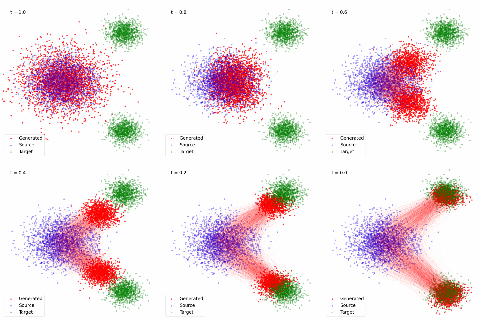
Figure 3: Trajectory of the samples following the reverse SDE with \(s_{\theta^\star}(x, t)\) computed using Eq. (23) for \(\alpha(t) = 1- t, \sigma(t) = t\).

4.2. Implementation: Sampling with Score based SDE

Here's a Python implementation that demonstrates how to convert a vector field into sore, and use the score for Reverse SDE based sampling. It was used to generate the animation in Figure 3 using the vector field in Figure 2.

import matplotlib.pyplot as plt
import matplotlib.animation as animation
import numpy as np
import torch
import math

def get_score_from_velocity(velocity, x, t):
    t = t.unsqueeze(-1)
    alpha_t, d_alpha_t = compute_alpha_t(t)
    sigma_t, d_sigma_t = compute_sigma_t(t)
    alpha_ratio = d_alpha_t / alpha_t
    lambda_t = d_sigma_t - alpha_ratio * sigma_t
    score = (alpha_ratio * x - velocity) / (sigma_t * lambda_t)
    return score

def get_drift_and_diffusion(x, t):
    t = t.unsqueeze(-1)
    alpha_t, d_alpha_t = compute_alpha_t(t)
    sigma_t, d_sigma_t = compute_sigma_t(t)
    alpha_ratio = d_alpha_t / alpha_t
    drift = alpha_ratio * x
    lambda_t = d_sigma_t - alpha_ratio * sigma_t
    diffusion = 2 * sigma_t * lambda_t
    return drift, diffusion

def euler_step(x, mean_x, t, model, dt, sde=False):
    w_cur = torch.randn(x.size()).to(x)
    t = torch.ones(x.size(0)).to(x) * t
    dw = w_cur * math.sqrt(dt)
    drift, diffusion = get_drift_and_diffusion(x, t)
    
    if not sde:
        velocity = drift - 0.5 * diffusion * get_score_from_velocity(model(x, t.unsqueeze(-1)), x, t)
        mean_x = x - velocity * dt
        x = mean_x 
    else:
        reverse_drift = drift - diffusion * get_score_from_velocity(model(x, t.unsqueeze(-1)), x, t)
        mean_x = x - reverse_drift * dt
        x = mean_x - torch.sqrt(diffusion) * dw
    return x, mean_x

@torch.no_grad()
def sample_sde(source_samples, model, device, steps=100, sde=False):
    model.eval()
    x = torch.tensor(source_samples, dtype=torch.float32).to(device)
    mean_x = x.clone()
    dt = 1.0 / steps
    
    for i in range(1, steps):
        t = torch.ones(x.size(0)).to(x) * (1 - i * dt)
        x, mean_x = euler_step(x, mean_x, t, model, dt, sde=sde)

    return x
        

5. References