You are hosting a grand birthday party at your house. Its your special day, and you have a sneaky plan in mind--eavesdropping on your friends' juicy gossips. You hide many microphones recorders all over the house. As your birthday unfolds, everything goes precisely as you had envisioned. But the next day, when you excitedly play back the recordings, you are met with a shocking revelation: all the voices are intertwined, its nearly impossible to decipher what anyone is saying.
This may sound like a plot from a mistery movie, but the solution to this perplexing problem lies in a powerful tool known as Independent Component Analysis (ICA) [1, 2, 3]. ICA isn't just confined to unmixing tangled audio sources; it can also be used to rectify image glitches, disentangle brain signals linked to various functions, pinpoint the factors influencing stock prices, and much more. In fact, by the end of this blog post, you will clearly understand how many of these daunting tasks can be solved in practice. Most importantly, you will hear what your friends say about you behind your back :).
The ICA model
Before we explore how to untangle the voices from the recorded audio, let's first understand how the magic happens behind the scenes. Imagine you have a microphone at your party – it's like an electronic ear that turns sound into electricity. We'll call the output of this microphone \(x_1\), and since it can capture sounds changing over time, we'll use \(x_1(t)\) to represent its value at any given moment.
If you have multiple microphones (let's say \(N\) of them), you'll have \(N\) different recordings, which we can call \(x_1(t), x_2(t), ..., x_N(t)\). These recordings are like snapshots of all the sounds happening around your party.
Now, imagine that amid the laughter and chatter, there are \(M\) individual sound sources. These could be your friends talking, music playing, or any other noise at your party. We'll represent these sound sources as \(s_1(t), s_2(t), ..., s_M(t)\). Our mission is to figure out what these sound sources are, given the recordings \(x_1(t), x_2(t), ..., x_N(t)\). But how are these recordings connected to the actual sounds?
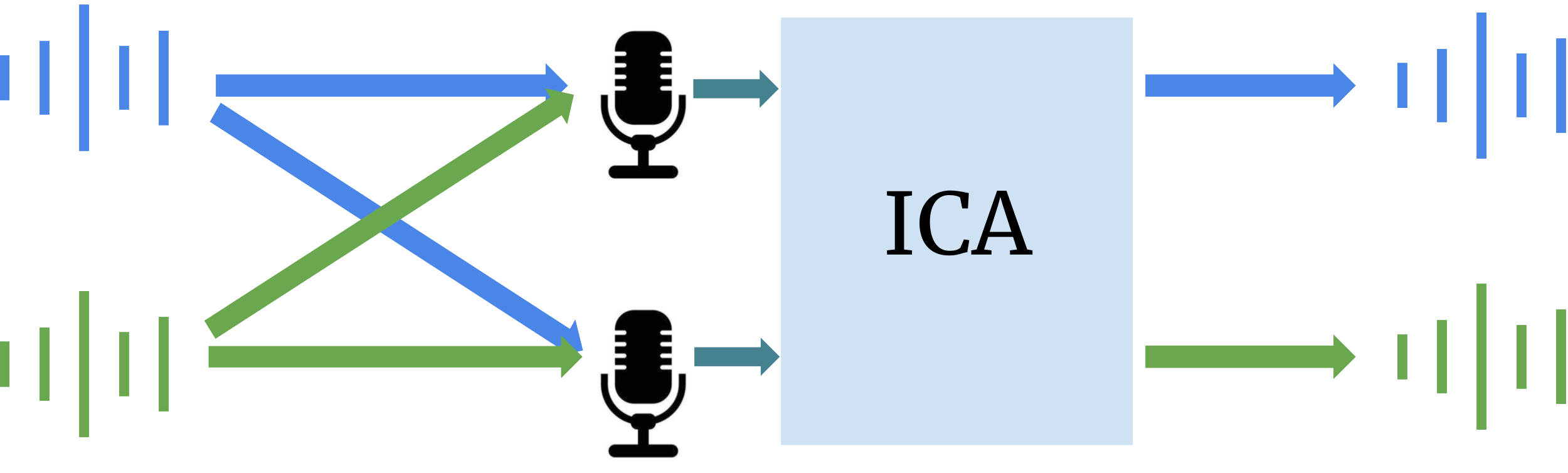
To make things simpler, let's say there are just two sound sources (\(M = 2\)) and two microphones (\(N = 2\)). A useful way to understand the relationship between recordings and sound sources is by thinking of it as a mix-up. Each recording (\(x_1(t)\) and \(x_2(t)\)) is like a blend of the two sound sources (\(s_1(t)\) and \(s_2(t)\)). It's like making a smoothie – you mix different ingredients to create a new flavor.
Mathematically, we can represent this mixing like this:
Here, the equations say that \(x_1(t)\) is a bit of \(s_1(t)\) (the first sound source) scaled by \(a_{11}\) and a bit of \(s_2(t)\) (the second sound source) scaled by \(a_{12}\). \(x_2(t)\) is a bit of \(s_1(t)\) scaled by \(a_{21}\) and a bit of \(s_2(t)\) scaled by \(a_{22}\). If \(a_{11}\) is small, it could mean that \(s_1(t)\) is far from the first microphone, and if \(a_{22}\) is large, it could mean that \(s_2(t)\) is close to the second microphone. So, in a nutshell, we're like detectives trying to un-mix the smoothie and discover the original flavors – our sound sources!
Now, considering Eq. (1) and (2), how can we retrieve the values of \(s_1(t)\) and \(s_2(t)\)? It seems like we have a system of linear equations here—two equations and two unknowns. However, let's take a moment to ponder. What are the values of \(a_{11}, a_{12}, a_{21},\) and \(a_{22}\)? As it turns out, all the variables on the right-hand side of equations (1) and (2) are also unknowns.
Is it even possible to solve this problem? There are two equations but six unknowns. Can we add more equations, i.e., add more microphones and turn it into a familiar linear programming problem? Unfortunately, it's not that straightforward. Adding more microphones would give rise to even more unknowns, e.g., \(a_{31}\), \(a_{32}\). In fact, generally, this problem remains unsolvable without additional insights. In ICA, we introduce a critical piece of information—a fundamental assumption about the nature of the sound sources.
To put it simply, the independence assumption means that the sound sources operate without influencing one another. For instance, if the sound sources represent different conversations, this assumption implies that one conversation doesn't interfere with the other, which seems reasonable.
Independence
Before we delve further, let's make a subtle adjustment to our equations:
We have dropped the time dependence of \(x_1,x_2, s_1, s_2\). Instead \(x_1,x_2, s_1, s_2\) are the so-called "random variables". A random variable is a useful concept in mathematics used to denote uncertain quantities. Think of them as placeholders for values that can change or vary unpredictably. In our case, these random variables represent the audio signals we're dealing with. Just like you can't always predict exactly what someone will say in a conversation or how loud they will be, these random variables capture the inherent unpredictability of the audio signals as they change over time. The use of random variables instead of time varying signal serves two purposes: (i) It allows us to deal with a wide range of signals (not necessarily time varying), e.g., images (ii) We can better understand the idea of independence and the remaining mathematical foundations underlying ICA.
Uniformly distributed sources
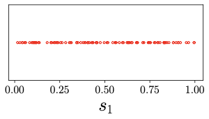
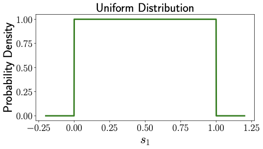
Let's make these concepts more tangible. Imagine that \(s_1\) is a like a random number you might pick between 0 and 1 on a spinner wheel. This number could be anything between 0 and 1, and each possibility is equally likely. Such a random number is known as uniform random variable. If we were to keep spinning the wheel multiple times and noting the numbers we get from \(s_1\), we'd collect data points like the ones you see in Figure 1.
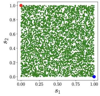
Now, let's think about a situation where both \(s_1\) and \(s_2\) are both uniform random variables. In this case, the samples from both \(s_1\) and \(s_2\) would look similar to what's shown in Figure 2. What's more, let's suppose that \(s_1\) and \(s_2\) are completely independent. In other words, the value of \(s_1\) doesn't affect what \(s_2\) will be, and vice versa. If we were to plot \(s_1\) on the \(x\)-axis and \(s_2\) on the \(y\)-axis, then the samples look like that in Fig. 3. We can see that no matter what value you pick for \(s_1\), you can't predict what \(s_2\) will be.
Now, let's specify some numbers for \(a_{11}, a_{12}, a_{21},\) and \(a_{22}\) and observe how \(x_1\) and \(x_2\) looks like. In Figure 3, we've chosen \(a_{11} = 2, a_{12} = 3, a_{21} = 4,\) and \(a_{22} = 1\). The dots that represent \(s_1\) and \(s_2\) in Figure 2 have transformed into different dots, representing \(x_1\) and \(x_2\) in Figure 3. But here's the cool part: if we look at the blue point \((1,0)\) and the red point \((0,1)\) in Figure 2, we can see how they become the new points:
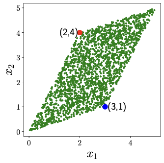
Blue point (s1,s2) = (1,0)
x1 = a11s1 + a12s2 = a11*1 + a12*0 = a11 = 2
x2 = a21s1 + a22s2 = a21*1 + a22*0 = a21 = 4
Red point (s1,s2) = (0,1)
x1 = a11s1 + a12s2 = a11*0 + a12*1 = a12 = 3
x2 = a21s1 + a22s2 = a21*0 + a22*1 = a22 = 1
Take a close look at those blue and red points; they're not just random dots. They happen to be the corners in the plot of \(x_1\) and \(x_2\). But here's the fascinating part: blue corresponds to \((x_1, x_2) = (a_{11}, a_{21})\), and red corresponds to \((x_1, x_2) = (a_{21}, a_{22})\).
This means that if our sound sources were random numbers (like spinning a wheel), and we could somehow pinpoint these special corner points from our recordings, we'd be able to figure out the exact values of \(a_{11}, a_{12}, a_{21},\) and \(a_{22}\)! By plugging these values into Eq. (3a) and (3b), we'd obtain two equations with two unknowns--a classic system of linear equations!
Beyond Uniform Distribution
The method we explored earlier works like a charm, but there's a catch—it only works when our sound sources act like random numbers picked uniformly, just like spinning a wheel. However, in real life, it's highly unlikely that the sounds we capture at your party follow such a neat pattern. So, we need to equip ourselves with more tools to develop a general Independent Component Analysis (ICA) solver that can handle a wider range of situations.
Gaussian Distribution
In Section 2.1, we looked at the uniform distribution, which gave us a good start. But there's another important distribution in the ICA world, and it's called the Gaussian distribution. This distribution has its own unique characteristics and is quite different from the uniform distribution.
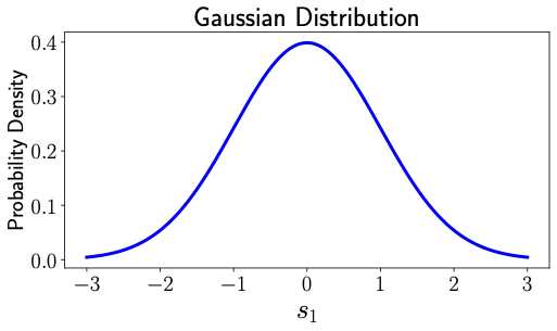
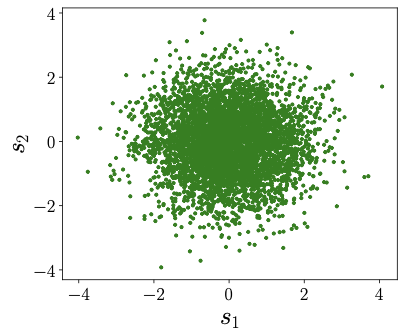
Imagine a bell-shaped curve like the one shown in Fig. 4 [Right]. That's what the probability density of a Gaussian distribution looks like. In contrast, the probability distribution of uniform distribution looks like Fig. 4 [Left]. In uniform distribution, all numbers between 0 and 1 had equal probability, therefore the same value of probability density in Fig. 4 [Left] in the interval between 0 and 1. But Gaussian distribution assigns different probabilities for different number as indicated by the values of probability density in Fig. 4 [Right]. When we take samples from a standard Gaussian distribution (similar to our uniform distribution samples in Fig. 2), they might look something like what you see in Fig. 5 [Left].
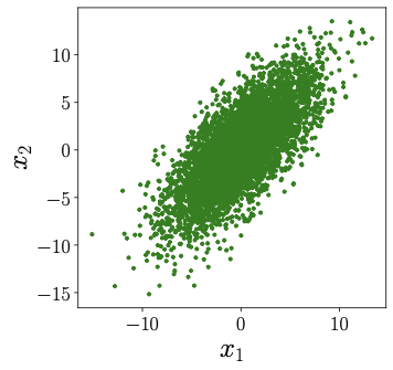
Now, let's talk about samples from \(x_1\) and \(x_2\), shown in Fig. 5 [Right]. Here's the thing: unlike the uniform distribution, when we observe these samples, it's incredibly tough to make any sense of \(a_{11}, a_{12}, a_{21},\) and \(a_{22}\). In fact, it's practically impossible to unmix the sources \(s_1\) and \(s_2\) from the recordings \(x_1\) and \(x_2\) if the sources themselves are Gaussian. That's why, in our ICA journey, we're going to make an explicit assumption--none of our sources are Gaussian distributed.
This assumption is pretty reasonable, considering that exciting signals like sound or images typically don't follow the Gaussian distribution. So, we're setting the stage to tackle the more complex cases we might encounter in the real world.
Vector Algebra
An important mathematical concept that will greatly aid our understanding of ICA is that of vectors and matrices. If you're already familiar with these concepts, feel free to skip ahead to the next sub-section. Vectors provide a concise way to represent and manipulate large sets of numbers. A \(N\)-dimensional vector, often represented by a boldface letter (e.g., \(\boldsymbol{v} \in \mathbb{R}^N\)), is defined as a collection of \(N\) scalars arranged in a single column with \(N\) rows as follows:
\[\boldsymbol{v} = \begin{bmatrix} v_1 \\ v_2 \\ \vdots \\ v_N \end{bmatrix}.\]
Similarly, a \(M \times N\) dimensional matrix, often represented by capitalized boldface letter (e.g., \(\boldsymbol{D}\)), is a collection of \(MN\) scalars, arranged into \(M\) rows and \(N\) columns as follows:
\[\boldsymbol{D} = \begin{bmatrix} d_{11} & d_{12} & \dots & d_{1N} \\ d_{21} & d_{22} & \dots & d_{2N} \\ \vdots & \vdots & \ddots & \vdots \\ d_{M1} & d_{M2} & \dots & d_{MN} \end{bmatrix}.\]
A transpose of a \(M \times N\) dimensional matrix, say \(\boldsymbol{D}\), is denoted by \(\boldsymbol{D}^{\mathsf{T}}\) and defined as the rearrangement of scalars in \(\boldsymbol{D}\) by swapping its columns and rows as follows:
\[\boldsymbol{D}^{\mathsf{T}} = \begin{bmatrix} d_{11} & d_{21} & \dots & d_{M1} \\ d_{12} & d_{22} & \dots & d_{M2} \\ \vdots & \vdots & \ddots & \vdots \\ d_{1N} & d_{2N} & \dots & d_{MN} \end{bmatrix}.\]
A multiplication between a \(M \times N\) dimensional matrix, say \(\boldsymbol{D\), and a \(N \times R\) dimensional matrix, say \(\boldsymbol{E}\), is denoted by \(\boldsymbol{D} \boldsymbol{E}\). The result, \(\boldsymbol{F} = \boldsymbol{D} \boldsymbol{E}\), is a new matrix of dimension \(M \times R\). We can express the elements of \(\boldsymbol{F}\) as
\[f_{mr} = d_{m1}e_{1r} + d_{m2}e_{2r} + \dots + d_{mN} e_{Nr}.\]
where \(f_{mr}\) is the scalar element on the \(m\)-th row and the \(r\)-th column of \(\boldsymbol{F}\). Note that the number of columns of the first matrix (here, \(\boldsymbol{D}\)) must be the same as the number of rows of the second matrix (here, \(\boldsymbol{E}\)) for multiplication \(\boldsymbol{D} \boldsymbol{E}\) to be possible. Multiplication between a matrix and a vector is defined in a similar fashion by treating the vector of \(N\) dimension as a matrix of \(N \times 1\) dimension. For example, \(\boldsymbol{D} \boldsymbol{v}\) represents multiplication of \(M \times N\)-dimensional vector \(\boldsymbol{D}\) with \(N\)-dimensional vector \(\boldsymbol{v}\), and has a dimension of \(M \times 1\). Similarly, \(\boldsymbol{v}^{\mathsf{T}}\) represents the transpose of \(\boldsymbol{v}\) with dimension \(1 \times N\).
ICA model using vector algebra
Using the new vector notation, we define \(\boldsymbol{s}\) as a vector that collects all our audio sources, i.e.,
\[\boldsymbol{s} = \begin{bmatrix} s_1 \\ s_2 \end{bmatrix}.\]
We similarly define the collection of all our recordings as vector \(\boldsymbol{x}\):
\[\boldsymbol{x} = \begin{bmatrix} x_1 \\ x_2 \end{bmatrix} \].
Finally, we arrange all the coefficients, \(a_{11}, a_{12}, a_{21}, a_{22}\), into a matrix (a two-dimensional vector) as follows:
\[\boldsymbol{A} = \begin{bmatrix} a_{11} & a_{12} \\ a_{21} & a_{22} \end{bmatrix}.\]
Under the new notation Eq. (1), (2) can be re-written concisely as follows:
\[\boldsymbol{x} = \boldsymbol{A} \boldsymbol{s}.\]
In fact, the above equation is unchanged even if we assume that we have a much larger number of sources and recordings (say \(N\)).
Now, remember our ultimate goal: to extract \(\boldsymbol{s}\) given \(\boldsymbol{x}\) given the information that the elements of \(\boldsymbol{s}\) are independent of each other. If \(\boldsymbol{x}\), \(\boldsymbol{A}\), and \(\boldsymbol{s}\) were scalar values (single numbers), i.e.,
\[x = as,\]
we could obtain \(s\) by multiplying \(x\) by \(a^{-1} = \frac{1}{a}\), i.e.,
\[s = a^{-1} x.\]
Thankfully, there is a similar concept for matrices--the matrix inverse, denoted by \(\boldsymbol{A}^{-1}\), which is another matrix. However, \(\boldsymbol{A}^{-1} \neq \frac{1}{\boldsymbol{A}}\), it has a slightly complex definition. Mainly, \(\boldsymbol{A}^{-1}\) is a matrix, which when multiplied with \(\boldsymbol{A}\) results in the identity matrix \(\boldsymbol{I}\), i.e.,
\[\boldsymbol{A}^{-1} \boldsymbol{A} = \boldsymbol{I} = \begin{bmatrix} 1 & 0 \\ 0 & 1 \end{bmatrix}.\]
Observe that if we left-multiply \(\boldsymbol{x}\) with \(\boldsymbol{A}^{-1}\), we obtain our sources!
\[\boldsymbol{A}^{-1}\boldsymbol{x} = \boldsymbol{A}^{-1} \boldsymbol{A} \boldsymbol{s} = \boldsymbol{I} \boldsymbol{s} = \begin{bmatrix} 1 & 0 \\ 0 & 1 \end{bmatrix} \begin{bmatrix} s_1 \\ s_2 \end{bmatrix} = \boldsymbol{s}.\]
Our primary objective is to find a matrix, let's call it \(\boldsymbol{B}\), that makes it equal to the inverse of \(\boldsymbol{A}\), denoted as \(\boldsymbol{A}^{-1}\). In other words, we seek a matrix \(\boldsymbol{B}\) such that:
\[ \begin{align*} \boldsymbol{B} \boldsymbol{x} &= \boldsymbol{s} \\ \implies \boldsymbol{B} \boldsymbol{A} \boldsymbol{s} &= \boldsymbol{s}. \end{align*} \]
Let's refer to the product of matrices \(\boldsymbol{B}\) and \(\boldsymbol{A}\) as \(\boldsymbol{R}\) for simplicity. Ideally, we'd like \(\boldsymbol{R}\) to be the identity matrix \(\mathbf{I}\), which would mean that all the sources are perfectly recovered. However, there are two inherent ambiguities that we can't avoid.
Firstly, we can't determine the exact order of the sources in \(\boldsymbol{s}\), which might lead to a permutation of sources in our results. To illustrate, let's say our ICA method gives us \(\widehat{\boldsymbol{s}} = \begin{bmatrix} \widehat{s}_1 \\ \widehat{s}_2 \\ \end{bmatrix}.\) It's possible that \(\widehat{s}_1\) corresponds to the audio source \(s_2\) instead of \(s_1\), and vice versa. This permutation occurs because shuffled sources still satisfy the independence condition. Thankfully, this doesn't pose a problem since our goal is to separate the voices or conversations.
Secondly, we won't be able to recover the exact amplitude or loudness of the audio sources. In other words, \(\widehat{s}_1\) might be equal to \(2s_2\), which says \(\widehat{s}_1\) could be twice as loud as \(s_2\). This scaling also conforms to the independence condition. Therefore, we can't expect \(\boldsymbol{R}\) to be an identity matrix. However, what we can expect is that \(\boldsymbol{R}\) takes on a particular form:
\[ \boldsymbol{R} = \begin{bmatrix} 0 & r_{12} \\ r_{21} & 0 \\ \end{bmatrix}. \]
In this form, \(r_{12}\) and \(r_{21}\) are non-zero scalars, while the other elements of \(\boldsymbol{R}\) are zero. This means that \(\widehat{s}_1 = r_{12} s_2\), a scaled version of \(s_2\), and \(\widehat{s}_2 = r_{21} s_1\), a scaled version of \(s_1\). In a nutshell, the recovered sources could be a combination of scaling and permutation of the original sources, but we've successfully separated and unmixed the original sources.
Non-Gaussianity for ICA
In the previous section, we found that the output of our ICA algorithm, denoted as \(\widehat{\boldsymbol{s}}\), can be expressed as linear combinations of the original sources: \(\widehat{s}_1 = r_{11} s_1 + r_{12} s_2\) and \(\widehat{s}_2 = r_{21} s_1 + r_{22} s_2\). In essence, this means that \(\widehat{s}_1\) and \(\widehat{s}_2\) are formed by scaling and summing the original sources. To effectively recover the audio sources, we require that each recovered source (e.g., \(\widehat{s}_1\)) should have only one of the coefficients (e.g., \(r_{11}\) or \(r_{12}\)) as non-zero. Achieving this can be accomplished through the utilization of the central limit theorem (CLT) [4].
The central limit theorem (CLT) is a fundamental concept in probability theory, stating that the sum of two or more independent random variables tends to have a distribution closer to Gaussian than a single random variable. In our context, when both \(r_{11}\) and \(r_{12}\) are non-zero, \(\widehat{s}_1\) tends to resemble a Gaussian distribution more closely than when only one of them is non-zero. This insight provides us with a method for evaluating whether a given random variable is likely to be a mixture of two or more independent random variables. The next section explores ICA methods based on the concept of promoting non-Gaussianity in estimated sources.
An ICA Algorithm
Various algorithms exist for estimating the ICA model, each offering a trade-off between accuracy, computational complexity, and the need for additional information. In this article, we'll delve into a widely adopted algorithm rooted in the principle of non-Gaussianity [3] introduced earlier.
To assess how closely a random variable resembles a Gaussian distribution, we can leverage unique properties of the Gaussian distribution that other distributions do not possess. For this purpose, let's define two vectors, \(\boldsymbol{b}_1\) and \(\boldsymbol{b}_2\), as follows:
\begin{align*} \boldsymbol{b}_1 = \begin{bmatrix} b_{11} \\ b_{12} \end{bmatrix}, \quad \boldsymbol{b}_2 = \begin{bmatrix} b_{21} \\ b_{22} \end{bmatrix}. \end{align*}
Consequently, we can express \(\widehat{s}_1 = \boldsymbol{b}_1^\top \boldsymbol{x}\) and \(\widehat{s}_2 = \boldsymbol{b}_2^\top \boldsymbol{x}.\)
One distinctive property of the Gaussian distribution is its high randomness compared to other distributions. In intuitive terms, randomness of a random variable refers to how spread out the probability density is or, equivalently, how spread out the random variable's samples are. The measure of randomness in a random variable is known as "entropy." For the purposes of this discussion, understanding the precise mathematical definition of entropy is not crucial. We will assume the existence of an oracle function \(\mathcal{H}\) that calculates the entropy of a random variable. For example, \(\mathcal{H}(s_1)\) would yield the entropy of \(s_1\). Let's denote a standard Gaussian random variable as \(g\). Since the Gaussian distribution exhibits the highest entropy, \(\mathcal{H}(g)\) will always be greater than \(\mathcal{H}(y)\) for any random variable \(y\) that is not Gaussian. We can now define a metric, \(\mathcal{J}\), as follows:
\[ \mathcal{J}(y) = \mathcal{H}(g) - \mathcal{H}(y). \]
Here, \(\mathcal{J}(y)\) quantifies the difference between the entropy of \(g\) and the entropy of \(y\). Notably, \(\mathcal{J}(y)\) is always a positive value and equals zero only when \(y\) follows a Gaussian distribution. Using this tool, we can compute the Gaussianity of \(\widehat{s}_1\) and \(\widehat{s}_2\) as:
\[ \mathcal{J}(\widehat{s}_1) = \mathcal{J}(\boldsymbol{b}_1^\top \boldsymbol{x}), \quad \mathcal{J}(\widehat{s}_2) = \mathcal{J}(\boldsymbol{b}_2^\top \boldsymbol{x}). \]
The ICA algorithm begins by initializing the elements of \(\boldsymbol{b}_1\) and \(\boldsymbol{b}_2\) with random values. Subsequently, it computes \(\mathcal{J}(\boldsymbol{b}_1^\top \boldsymbol{x})\) and \(\mathcal{J}(\boldsymbol{b}_2^\top \boldsymbol{x})\). The values of \(\boldsymbol{b}_1\) and \(\boldsymbol{b}_2\) are then updated iteratively to reduce \(\mathcal{J}(\boldsymbol{b}_1^\top \boldsymbol{x})\) and \(\mathcal{J}(\boldsymbol{b}_2^\top \boldsymbol{x})\). This update process can be executed using various methods such as gradient descent or Newton's iteration. In the FastICA algorithm, an approximate form of Newton's iteration is employed. These update steps continue until no significant changes are observed in the values of \(\boldsymbol{b}_1\) and \(\boldsymbol{b}_2\), signifying convergence. Once the algorithm has converged, we can utilize the resulting \(\boldsymbol{b}_1\) and \(\boldsymbol{b}_2\) to extract the audio sources as follows:
\begin{align*} \widehat{s}_1(t) &= b_{11} x_1(t) + b_{12} x_2(t), \\ \widehat{s}_2(t) &= b_{21} x_1(t) + b_{22} x_2(t). \end{align*}
This extraction process effectively separates and recovers the original sources from the mixed recordings.
Try it out !
Now that you have a basic understanding of the ICA problem and a simple algorithm to solve it, here is a python notebook (Prepared by my colleague Jiahui Song) to help get a better understanding and hands on experince: ICA Colab Notebook
Conclusion
If you have made it to this point, you hopefully understand the problem of ICA, basic assumptions for solving ICA, and a basic algorithm for solving ICA. If you are interested in exploring further and going deeper into this problem, you can explore an accessible paper that delves into the subject [3]. This understanding can also serve as a solid foundation for delving into more intricate and general tasks in the fields of machine learning and AI, including nonlinear ICA [6], latent variable models [5], disentanglement, and other key elements of the deep learning domain. Enjoy your exploration!
References
[1] Jutten, Christian, and Jeanny Herault. "Blind separation of sources, part I: An adaptive algorithm based on neuromimetic architecture." Signal processing 24.1 (1991): 1-10.
[2] Comon, Pierre. "Independent component analysis, a new concept?." Signal processing 36.3 (1994): 287-314.
[3] Hyvärinen, Aapo, and Erkki Oja. "Independent component analysis: algorithms and applications." Neural networks 13.4-5 (2000): 411-430.
[4] "Central Limit Theorem." Wikipedia, Wikimedia Foundation, 25 Oct. 2023, en.wikipedia.org/wiki/Central_limit_theorem.
[5] Goodfellow, Ian, et al. "Deep learning." An MIT Press book (2016).
[6] Hyvärinen, Aapo, and Petteri Pajunen. "Nonlinear independent component analysis: Existence and uniqueness results." Neural networks 12.3 (1999): 429-439.